Spectral sampling from Gaussian processes
The Bayesian multi-objective optimization algorithm TSEMO [Bradford2018] uses Thompson sampling of the surrogate Gaussian process model. In order to sample a function from a Gaussian process posterior, an approximate method using spectral sampling [Hernandez2014] is employed. In the following we implement this method in Python.
There is also a nice python package, called pyrff that implements spectral sampling, but I found out only later.
Theory
Blochner's theorem shows that any stationary kernel \(k(x, x') = k(x - x', 0) = k(r)\) and its spectral density \(s(w)\) are Fourier duals
By normalizing, the spectral density becomes a probability density \(p(w) = s(w) / \alpha\) where \(\alpha\) is equal to the kernel variance. Hence, we can write the integral of \(k(r)\) as an expectation
where \(\zeta(x) = e^{-i w^T x}\) is a feature mapping. Since the integral is real, we can substitute by cosine expressions. It can be shown that \(\zeta(x) = \sqrt{2 \alpha} \cos(w^T x + b)\) satisfies the equation. Furthermore, the expectation can be approximated via Monte Carlo sampling.
where \([W]_i \sim p(w)\) and \([b]_i \sim U(0, 2\pi)\) are \(m\) stacked Monte Carlo samples.
The feature mapping allows us to approximate GP sample functions \(f(x) \sim GP(m(x), k(x,x'))\) with a linear model
Without data \(\mu_\theta=0, V_\theta=1\), whereas with data
where \([Z]_i = \zeta(x_i)\) consists of the stacked feature mappings evaluated at the inputs of the data.
The probability density associated with Matérn kernels takes the form of a multivariate t-distribution with \(\nu\) degrees of freedom. For the squared exponential (RBF) kernel (\(\nu \leftarrow \infty\)), the t-distribution reduces to the normal distribution.
And that's it.
Implementation
Note 1: The inversion of matrix \(A\) can leads to numerical problems for \(m > 5\). We do the usual thing of using the Cholesky decomposition \(A = L^T L\), since \(A\) is symmetric and positive semidefinite. Due to numerical inaccuracies, we may need to add some some jitter to the diagonal elements of \(A\) to enforce positive semidefiniteness. This is handled in GPy's utility functions.
Note 2: In order to generalize to other Matern kernels (GPy supports \(\nu\) = ½, 3/2 and 5/2) we need to sample from a t-distribution. We can use the univariate t-distribution provided by scipy as the covariance matrix \(\Lambda\) is diagonal, meaning that the \(d\) samples for the individual input dimensions are uncorrelated and can be independently sampled.
class SpectralSampling:
    def __init__(self, gp, m=30):
        self.gp = gp

        # Create a random spectral feature mapping
        d = gp.input_dim
        if isinstance(gp.kern, GPy.kern.RBF):
            # W = np.random.randn(m, d) / gp.kern.lengthscale
            W = np.random.randn(m, d) / gp.kern.lengthscale
        else:
            if isinstance(gp.kern, GPy.kern.Exponential):
                ν = 1 / 2
            elif isinstance(gp.kern, GPy.kern.Matern32):
                ν = 3 / 2
            elif isinstance(gp.kern, GPy.kern.Matern52):
                ν = 5 / 2
            else:
                raise ValueError(f"Unknown kernel {gp.kern}")
            W = scipy.stats.t.rvs(ν, size=(m, d)) / gp.kern.lengthscale
        b = 2 * np.pi * np.arange(0, m).reshape(-1, 1) / m
        self.ζ = lambda x: (2 * gp.kern.variance / m) ** 0.5 * np.cos(W @ x.T + b)

        # Calculate the posterior mean and variance
        var_noise = gp.likelihood.variance
        Z = self.ζ(gp.X)
        A = Z @ Z.T + np.diag(var_noise)
        L = GPy.util.linalg.jitchol(A)
        Ainv, _ = GPy.util.linalg.dpotri(L)
        self.μθ = (Ainv @ Z @ gp.Y).ravel()
        self.Vθ = Ainv * var_noise
        self.Vθ /= m**0.5  # ad-hoc scaling, otherwhise the posterior variance increases with increasing m

    def predict(self, x):
        """Posterior mean and variance"""
        Z = self.ζ(x)
        μ = Z.T @ self.μθ
        V = Z.T @ self.Vθ @ Z
        return μ, np.diagonal(V)

    def sample(self):
        """Random posterior sample *function*"""
        θ = np.random.multivariate_normal(self.μθ, self.Vθ)
        return lambda x: self.ζ(x).T @ θ
def plot_cases(gps, m=10, exact_samples=None, spectral_samples=None):
    n = len(gps)
    fig, axs = plt.subplots(1, n, figsize=(6 * n, 5), sharey=True)
    fig.subplots_adjust(wspace=0.05)
    axs[0].set_ylabel('$y$')

    for ax, gp in zip(axs, gps):
        title = f"{gp.kern.name}, $\lambda$={gp.kern.lengthscale[0]:.1f}, $\sigma_f$={gp.kern.variance[0]**.5:.1f}, $\sigma_n$={gp.likelihood.variance[0]**.5:.2f}"
        gp.plot(ax=ax)
        ax.set(xlim=(0, 1), ylim=(-3.5, 3.5), xlabel='$x$', title=title)

        # exact samples points
        if exact_samples is not None:
            gp.plot_samples(ax=ax, samples=exact_samples)

        # approximate sample functions, via spectral sampling
        if spectral_samples is not None:
            ss = SpectralSampling(gp, m=m)

            # posterior mean and covariance
            x = np.linspace(0, 1, 101)[:, None]
            μ, V = ss.predict(x)
            ax.plot(x.ravel(), μ, color='C1', lw=2, ls='--')
            ax.fill_between(x.ravel(), μ - 2 * V**.5, μ + 2 * V**.5, alpha=0.2, color='C1')

            # individual samples
            [ax.plot(x.ravel(), ss.sample()(x), 'C1', lw=1) for i in range(spectral_samples)]
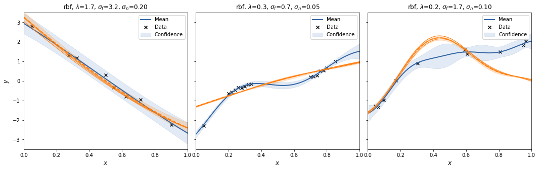
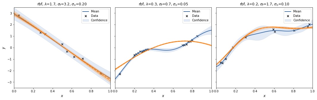
Example: Approximating an RBF kernel
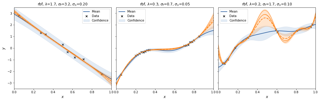
In the following we consider three examples of 1-dimensional RBF kernels with varying lengthscales, amplitudes and noise. For each kernel we sample a number of data points, fit a GP with the true kernel, and draw same approximate sample functions from the posterior.
np.random.seed(42)

# data from linear model, fitted with GP using RBF kernel
x = np.array([0.05, 0.275, 0.325, 0.5, 0.55, 0.625, 0.7125, 0.9]).reshape(-1, 1)
y = - 6 * x + 3 + np.random.randn(*x.shape) * 0.2
gp1 = GPy.models.GPRegression(x, y, kernel=GPy.kern.RBF(1))
gp1.kern.variance = 10
gp1.kern.lengthscale = 1.7
gp1.likelihood.variance = 0.04

# data from quadratic model, fitted with GP using RBF kernel
x = np.array([0.05, 0.2, 0.22, 0.24, 0.26, 0.28, 0.3, 0.32, 0.34, 0.7, 0.72, 0.74, 0.76 ,0.78, 0.8, 0.85]).reshape(-1, 1)
y = 25 * (x - 0.5) ** 3 + np.random.randn(*x.shape) * 0.05
gp2 = GPy.models.GPRegression(x, y, kernel=GPy.kern.RBF(1))
gp2.kern.variance = 0.5
gp2.kern.lengthscale = 0.3
gp2.likelihood.variance = 0.05**2

# data sampled from GP with RBF kernel and fitted with same GP
k = GPy.kern.RBF(1, lengthscale=0.2, variance=3)
x = np.random.rand(10, 1)
y = np.random.multivariate_normal(mean=np.zeros(len(x)), cov=k.K(x, x))[:, None]
y += -1 + np.random.randn(*y.shape) * 0.2
gp3 = GPy.models.GPRegression(x, y, kernel=k, noise_var=0.01)

plot_cases([gp1, gp2, gp3], exact_samples=5)

For each case we create a SpectralSampling object with a random feature mapping using m=3 samples from the kernels' spectral density. We plot the posterior mean and 95% interval (excluding the noise variance!) for that specific feature mapping, and sample 3 functions from it (orange).
With m=3 the spectral sampling procedure underfits.
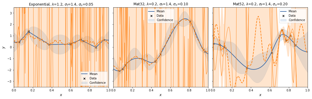
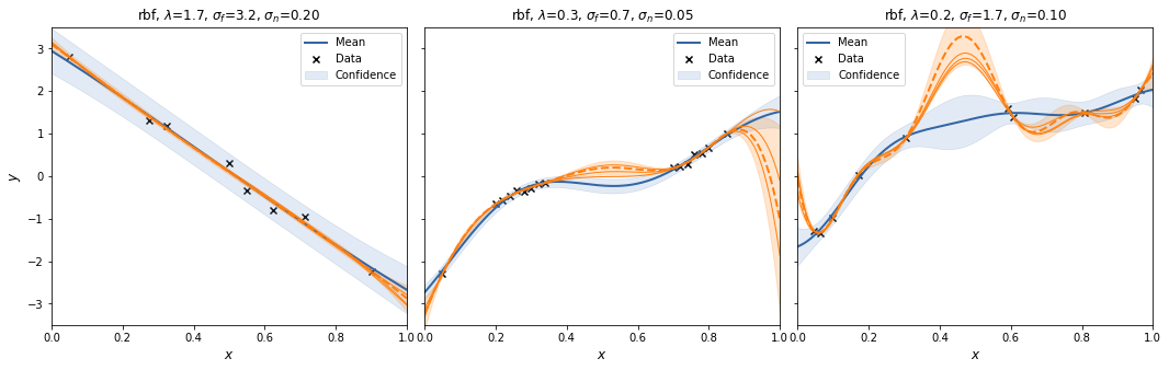
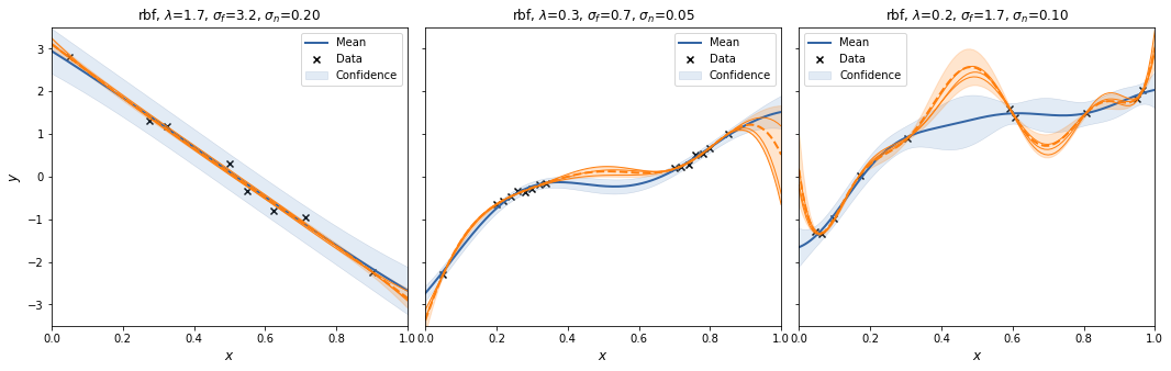
To see the effect of randomness of the feature mapping, we repeat to procedure a couple of times.
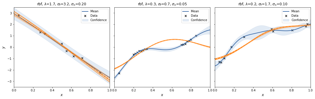
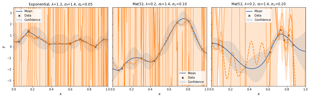
Let's try that with m=30.
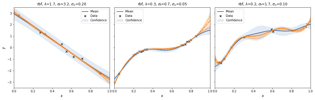
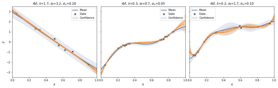
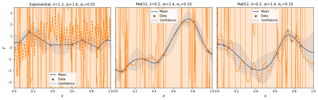
And with m=300.
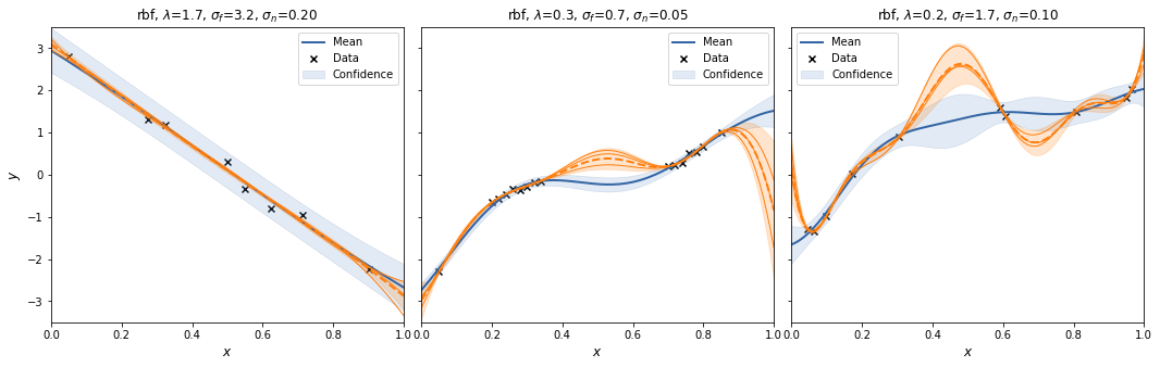
Interestingly, the spectral sampling procedure does not seem to converge to the GP posterior with increasing \(m\), but actually develops an oscillatory behaviour in between supporting data points, and when extrapolating.
Also, I added a scaling factor to \(V_\theta\) as otherwise the posterior variances increases with increasing \(m\).
Example: Approximating other Matern kernels
For each kernel we draw random data from the kernel and then plot the posterior GP along with some normal and spectral samples.
np.random.seed(42)

# Matern 1/2 kernel
k = GPy.kern.Exponential(1, lengthscale=1.2, variance=2)
x = np.random.rand(10, 1)
y = np.random.multivariate_normal(mean=np.zeros(len(x)), cov=k.K(x, x))[:, None]
y += np.random.randn(*y.shape) * 0.05
gp4 = GPy.models.GPRegression(x, y, kernel=k, noise_var=0.05**2)

# Matern 3/2 kernel
k = GPy.kern.Matern32(1, lengthscale=0.2, variance=2)
x = np.random.rand(10, 1)
y = np.random.multivariate_normal(mean=np.zeros(len(x)), cov=k.K(x, x))[:, None]
y += np.random.randn(*y.shape) * 0.1
gp5 = GPy.models.GPRegression(x, y, kernel=k, noise_var=0.1**2)

# Matern 5/2 kernel
k = GPy.kern.Matern52(1, lengthscale=0.2, variance=2)
x = np.random.rand(10, 1)
y = np.random.multivariate_normal(mean=np.zeros(len(x)), cov=k.K(x, x))[:, None]
y += np.random.randn(*y.shape) * 0.2
gp6 = GPy.models.GPRegression(x, y, kernel=k, noise_var=0.2**2)

plot_cases([gp4, gp5, gp6], exact_samples=5)

Now let's look at some spectral samples. Here we see a strong variance in the results. Either something is wrong in the implementation, or sampling from the t-distribution for few degrees of freedom needs a very large number of samples to the increased variance when sampling from a strongly tailed distribution.